Company at the perfectly competitive market
Here we start with the analysis of a firm’s behavior at the perfectly competitive market. Firm is taking a market price p as given and beyond its control (see Robinson (1934) and Stigler (1957) for a seminal discussion of the basic assumptions underlying perfect competition and its methodological development). The demand it faces is hence given by:

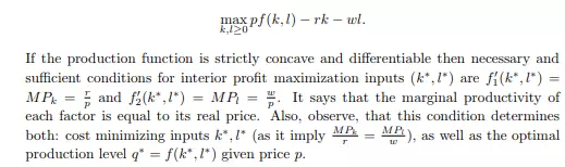
with F C > 0 that are sunk. Then condition ’price equal to marginal costs’ is still necessary, but not sufficient unless π ∗ = pq∗ − V C(q ∗ ) − F C ≥ −F C. This says that profit must exceed profit of producing zero (−F C). And that yields condition: p ≥ V C(q ∗ ) q ∗ = AV C(q ∗ ). The price level at which p = AV Cmin is called a shutdown level as the company would be better off closed. For the case, when the fixed costs are nonsunk the condition becomes π ∗ = pq∗ − V C(q ∗ ) − F C ≥ 0 or p ≥ AT C. That is, as the nonsunk costs are avoidable, then firm would continue production until profits are positive. Some costs are sunk in the short run, but in the long run most costs become nonsunk. Hence p ≥ AV C(q ∗ ) is a condition for firm’s positive operations in the short run, while p ≥ AT C(q ∗ ) in the long run. The intermediate cases, where some fixed costs are sunk, while others not, can also be considered. Observe that condition p = MC(q ∗ ) implicitly defines a supply function S(p) by p = MC(S(p)) with T C00(S(p)) ≥ 0 as long as (short or log run) operating conditions are satisfied. Hence the inverse of marginal costs defines a (short or long run) firm’s supply curve. In the analysis so far we have assumed that T C function was derived from company costs minimization problem. Still, a direct analysis is possible. We study it now. Consider a profit maximization problem of a firm with production function f taking prices p of output and inputs w, r as given:
Competitive equilibrium and welfare
In the previous section we have derived a supply curve S of a firm at the perfectly competitive market. If we sum supplies of all m firms we obtain a market or aggregate supply: Pm j=1 Sj (p). Similarly in the previous chapter we obtained an
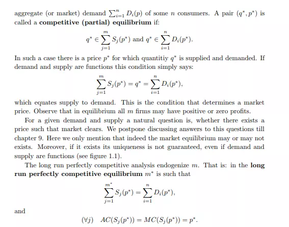
Interpreting: in the long run competitive equilibrium the profits of all companies are zero. This must hold since, as if they were positive, some new companies could appear, enter the market and reduce them. We now move to welfare analysis of competitive equilibrium. For this reason assume there is a representative consumer with quasilinear, differentiable utility function u(x) + y, where y is simply money left for purchase of other goods, and it is the market for good x that is under study. We already know that demand for x is given implicitly by u 0 (D(p)) = p, where p is a price of x. Assume also that a total cost function of producing x is given by T C with T C00(·) > 0 and T C(0) = 0. Then supply of x is given implicitly by T C0 (S(p)) = p. In the competitive equilibrium we hence have:
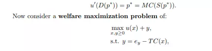
where ey is an initial endowment in good y. This problem maximizes utility of a representative consumer under the feasibility constraint, and yields a first order condition for interior solution: