The consumer, so it is said, is the king. . . each is a voter who uses his money as votes to get the things done that he wants done ñPaul Samuelson, Economics (1948)

There is a small collection of big issues that remain in connection with the consumer. These focus on the consumerís interaction with the surrounding economic environment and cover the following:

Determination of incomes.

Just as the market determines the prices of the goods that consumer buy, so too it may determine a large part, if not all, of their incomes. Instead of receiving a lump sum, members of a household generate their income by trading in the market. The price system therefore has a fuller rÙle in ináuencing consumer behaviour than we accorded it in the simple model of chapter 4. (section 5.2)  Supply by households. Implicit in the issue of income determination is the idea that the household will be selling goods and services to the market, as well as buying. We need to see how the basic analysis of the consumer can be adapted to include this phenomenon. (section 5.3)

Household production.

Not all the objects in the utility function are on sale in the market. Instead the household may perform activities similar to that of a Örm by buying market goods not for their own sake but in order to use them as inputs in the production of the things that it really wants

Aggregation over goods and households.

Analysing the choices of a single agent over bundles of n commodities is a useful base on which to build a theory of consumersíbehaviour. However the extension of our analysis to more general economic models suggests ñand data limitations usually require ñ(i) that we consider broadly deÖned groups of commodities and (ii) that we analyse demands by groups of consumers. (sections 5.5 and 5.6) We begin with a re-examination of the consumerís budget constraint. 5.2 The market and incomes So far we have taken the consumerís budget constraint to be of the form (4.5) where y is an exogenously given number of dollars, euros or pounds. We have assumed that the consumerís income is like a state pension for the elderly or pocket money for the young. This is clearly somewhat restrictive. In order to make progress we need to use something like that depicted in the right-hand panel of Figure 4.2. To do this we introduce an elementary system of property rights. An individual owns R1; R2; :::; Rn of commodities 1; 2; :::; n; some of the Ri could be zero (if the consumer possesses none of that commodity) but no Ri can be negative. The personís income comes from selling in the market some of the resources that he owns. Given market prices p1; p2; :::; pn we have

Obviously other, speciÖcations of income are possible. For example, we could also have a hybrid case where the consumer had some income from the sale of resources, some shares in the proÖts of Örms (we will be dealing with that in chapter 7) and some income Öxed in money terms; but (5.1) is rich enough for present purposes. Obviously, too, we could translate all this from the case where the consumer is an individual to that where the consumer is a household.

Supply by households

Now the consumerís problem can be expressed: ìmaximise utility subject to the constraint that expenditure is less than or equal to the value of resourcesî. To

Obviously a change in prices will in general induce a change in resource incomes as well as changes in consumption demand. Consider the implications of the demand function (5.4). Obviously if, for some i, the optimum value of x i is greater than Ri we have a fairly conventional case of consumption demand for this good; but if x i < Ri (and pi > 0) then an amount Ri x i is being supplied to the market. Factor supply by households can thus be treated symmetrically with consumption demand by households within this simple model. Now let us examine the comparative statics of these demand functions (since each Ri is Öxed, to get the e§ect on the supply in each case below, simply put a minus sign in front). First consider the e§ect on consumer demand of an increase in the endowment Rj : this simply augments the personís income by an amount proportional to pj . So the net result is a simple modiÖcation of the income e§ect that we introduced above

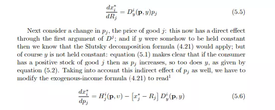
6) Notice the importance of the sign of the term [x j Rj ] in (5.6). Let us suppose that good i (oil) is a normal good (so that the term Di y is positive). If the price of oil goes up and you are net oil demander (so x j > Rj ) this event is bad news and it is clear from (5.4) that the impact on demand is similar to the exogenous income case; but if you are a net oil supplier (for whom x j < Rj ) this is good news and the income e§ect goes in the other direct

The ofer curve

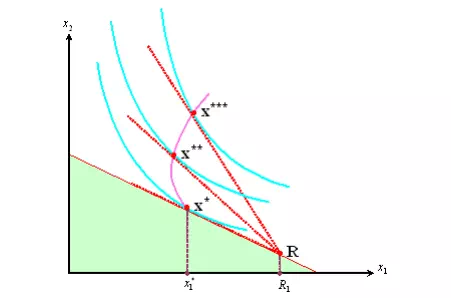
In cases where Rj x j > 0 ñwhere the individual is a net supplier ñyou may get responses to price changes that might appear to be strange. To see this, look at Figure 5.1 that introduces a useful concept for cases where consumersíincomes are determined endogenously, the o§er curve. This is the set of consumption bundles demanded (trades o§ered) at di§erent prices. The initial resource endowment is denoted R and the original budget constraint is indicated by the shaded triangle: clearly the optimal consumption bundle is at x where the person supplies an amount R1 x 1 in order to buy extra units of commodity 2. If the price of good 1 rises (equivalently, the price of good 2 falls) then the optimum shifts to x and then to x . Notice that, while the consumption of good 2 increases steadily, the supply of good 1 at Örst rises and then falls. The locus of equilibrium points (on which x ; x and x lie) is the o§er curve and its shape clearly depends on the position of R