Equal-product curves are similar to the indifference curves of the theory of consumer’s behaviour. An equal-product curve represents all those input combinations which are capable of producing the same level of output. The equal-product curves are thus contour lines which trace the loci of equal outputs. These equal-product curves are also known as isoquants (meaning equal quantities) and iso-product curves. Since ah equal-product curve represents those combinations of inputs which will be capable of producing an equal quantity of output, the producer would be indifferent between them as such. Therefore, another name which is often given to the equal-product curves is production-indifference curve’. The concept of equal-product curves can be easily understood from Table 1. It is presumed that two factors X and Y are being employed to produce a product.
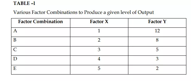
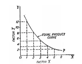
Each of the factor combinations A, B, C, D and E produces the same level of output, say, 20 units. To start with, factor combination A consisting of 1 unit of factor X and 12 units of factor Y produces the given 20 units of output. Similarly, combination B consisting of 2 units of X and 8 units of Y, combination G consisting of 3 units of X and 5 units of Y, combination D consisting of 4 units of X and 3 units of Y, and combination E consisting of 5 units of X and 2 units of Y are capable of producing the same amount of output, we have plotted all these combinations and by joining them we obtain the equal-product curve showing that every combination represented on it can produce 20 units of output.
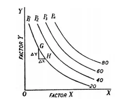
Though equal product curves are similar to the indifference curves of the theory of consumer’s behaviour, yet there is one important difference between the two. An indifference curve represents all those combinations of two goods which provide the same satisfaction or utility to a consumer but no attempt is made to specify the level of satisfaction or utility it stands for. This is so because the measurement of satisfaction or utility in unambiguous terms is not possible. That is why we usually label indifference curves by ordinal numbers as I, II, III, etc., indicating that a higher indifference curve represents a higher level of satisfaction than a lower one, but the information as to by how much one level of satisfaction is greater than another is not provided. On the other hand, we can label equal product curves in the physical units of output without any difficulty. Production of a good being a physical phenomenon lends itself easily to absolute measurement in physical units. Since each equal product curve represents specified level of production, it is possible to say by how much one equal-product curve indicates greater or less production than another. In Fig. 2 we have drawn an equal-product map or isoquant map with a set of four equal product curves which represent 20 units, 40 units, 60 units and 80 units of output respectively. Then, from this set of equal-product curves it is very easy to judge by how much production level on one equal-product curve is greater or less than on another.
MARGINAL RATE OF TECHNICAL SUBSTITUTION
Marginal rate of technical substitution in the theory of production is similar to the concept of marginal rate of substitution in the indifference curve analysis of consumer’s demand. Marginal rate of technical substitution indicates the rate at which factors can be substituted at the margin without altering the level of output. More precisely, marginal rate of technical substitution of factor X for factor Y may be defined as the amount of factor Y which can be replaced by one unit of factor X, the level of output remaining unchanged.
The concept of marginal rate of technical substitution can be easily understood from the Table 2. Each of the input combinations A, B, C, D and E yields the same level of output. Moving down -the table from combination A to combination B, 4 units of Y are replaced by 1 unit of X in the production process without any change in the level of output
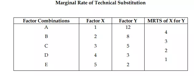
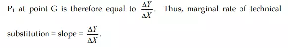
Therefore, the marginal rate of technical substitution is 4 at this stage switching from input combination B to input combination G involves the replacement of 3 units of factor Y by an additional unit of factor X, output remaining the same. Thus, the marginal rate of technical substitution is now 3. Likewise, marginal rate of technical substitution between factor combinations G and D is 2, and between factor combinations D and E is 1. The marginal rate of technical substitution at a point on the equal product curve can be known from the slope of the equal product curve at that point. Consider a small movement down the equal product curve P1 from G to H in Fig 2 where a small amount of factor Y, say DY, is replaced by an amount of factor X, say DX without any loss of output. The slope of the isoproduct curve
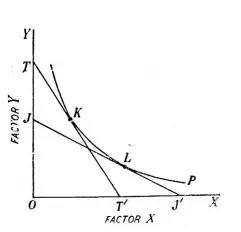
Slope of the equal product curve at a point and hence the marginal rate of technical substitution (MRTS) can also be known by the slope of the tangent drawn on the equal product curve at that point. In Fig 3 the tangent TT’ is drawn at point K on *he given equal product curve P. The slope of the tangent TT’ is equal to OT’ OT . Therefore, the marginal rate of technical substitution at point K on the equal product curve P is equal to OT’ OT . JJ’ is the tangent to point L on the equal product curve P. Therefore, the marginal rate of technical substitution at point L is equal to OJ/OJ.
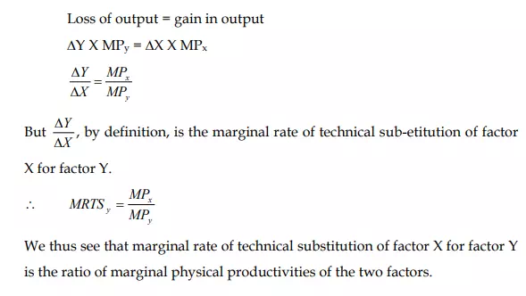
An important point to be noted about the marginal rate of technical substitution is that it is equal to the ratio of the marginal physical products of two factors. Since, by definition, output remains constant on the equal product curve the loss in physical output from a small reduction in factor Y will be equal to the gain in physical output from a small increment in factor X. The loss in output is equal to the marginal physical product of factor Y (MPV) multiplied by the amount of reduction in Y. The gain in output is equal to the marginal physical product of factor X (MP.) multiplied by the increasement in X