If we think about the indifference curves in a slightly different way, we see that MRS describes marginal benefit. Since MRS represents the maximum amount of y we are willing to give up in exchange for one unit of x, it also represents how much value our consumer places on x in terms of y.
This means the indifference curve tells us the marginal benefit of good x in terms of good y, and the budget line tells us the marginal cost of good x in terms of good y. As discussed in Topic 1, using marginal analysis, our consumer will continue to purchase more of a good until the marginal benefit is equal to the marginal cost. This means
if MRS > Px/Py, the consumer will consume more x and less y.
If MRS < Px/Py, the consumer will consume less x and more y.
If MRS = Px/Py, the consumer will not change their consumption.
Recall that MRS is the slope of the indifference curve, and Px/Py is the slope of the budget line. This means that if the slope of the indifference curve is steeper than that of the budget line, the consumer will consume more x and less y.
Figure 6.3a shows José’s budget line and possible indifference curves. As Point A, MRS is greater than Px/Py, so José should consume more x and less y to maximize his utility.
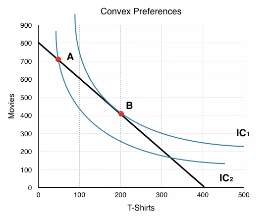
Moving along the budget line (shown in black), we see this action indeed allows José to consume on a higher indifference curve. At point B, MRS = Px/Py, so this is the utility maximizing point, given José’s constraints. Notice that since Point A and Point B are on the same budget line, José could increase utility without a change in expenditures.
In summary, the consumer will consume at the point where the indifference curve and the budget line are tangent, meaning the slopes are equal.
When Prices Changes
We now have all the pieces to develop our model for consumer theory. In Topic 3, we examined the law of demand, which showed that as the price increased our quantity demanded of the good decreased. Now, let’s look at how our consumption choices react to a change in price based on our indifference curve and budget line.
Consider a market with 100 consumers like José, each with budgets of $56 and preferences as illustrated in Figure 6.3b.
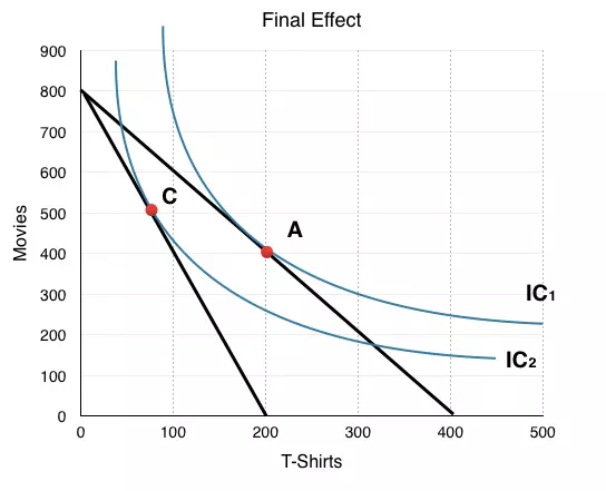
The graph shows the final effect of a price increase on T-shirts. Suppose T-shirts have increased from $14 to $28.
The easiest way to graph a price change is to assume José spends all of his money on T-shirts to see how the intercept will change. Following the price increase, he can only purchase 2 T-shirts. ($56 budget / $28/T-shirt) Because we are imagining a market with 100 consumers like José, all in all, 200 T-shirts will be bought. The price increase causes the budget line to pivot inwards and changes the price ratio from Px/Py = 2 to Px/Py = 4.
Since we know the price of movies has not changed, we know that José can still purchase 8 movies and can show the new graph with our knowledge of these points.
In our example, this causes consumers to change consumption from 200 T-Shirts and 400 Movies (Point A) to around 70 T-Shirts and 500 Movies (Point C). Why is this the case? Can we tell from this graph whether the two goods are compliments or substitutes? Normal or inferior?
To answer these questions, we can decompose the consumer’s response into two parts:
1. The substitution effect (SE): isolates the effect of the change in relative prices, by holding well-being constant.
-Draw a BL with the same slope as the new one, but draw it touching the original IC at the point of tangency.
-The movement from the old optimal consumption point to this new tangency point is the SE.
2. The income effect (IE): isolates the effect of the change in purchasing power (well-being), holding prices constant.
-Draw the final BL associated with the price change.
-The movement from the consumption point on the BL drawn in the SE to the optimal point on the final BL is the IE.


Comments are closed.